Time Domain
With the files in the folder SFS_time_domain you can simulate snapshots in time
of an impulse originating from your WFS or NFC-HOA system.
In the following we will create a snapshot in time after 5 ms for a broadband virtual point source placed at (0 2 0) m for 2.5D NFC-HOA.
conf = SFS_config;
conf.dimension = '2.5D';
conf.plot.useplot = true;
% sound_field_imp_nfchoa(X,Y,Z,xs,src,t,conf)
[p,x,y,z,x0] = sound_field_imp_nfchoa([-2 2],[-2 2],0,[0 2 0],'ps',0.005,conf);
%print_png('img/sound_field_imp_nfchoa_25d.png');
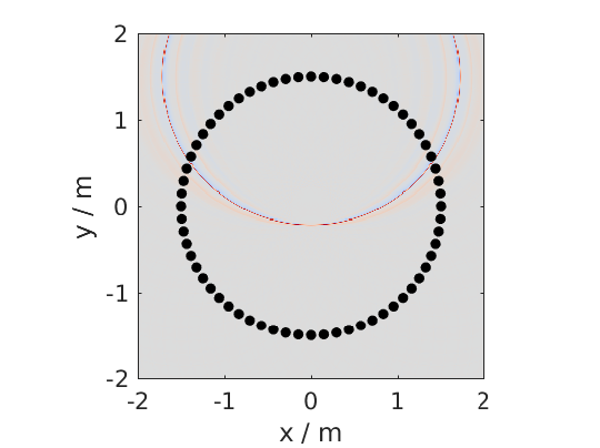
Fig. 18 Sound pressure of a broadband impulse point source synthesized by 2.5D NFC-HOA. The point source is placed at (0,2,0) m and the time snapshot is shown 5 ms after the first secondary source was active.
The output can also be plotted in dB by setting conf.plot.usedb = true;.
In this case the default color map is changed and a color bar is plotted
in the figure. For none dB plots no color bar is shown in the plots. In
these cases the color coding goes always from -1 to 1, with clipping of
larger values.
conf.plot.usedb = true;
plot_sound_field(p,[-2 2],[-2 2],0,x0,conf);
%print_png('img/sound_field_imp_nfchoa_25d_dB.png');
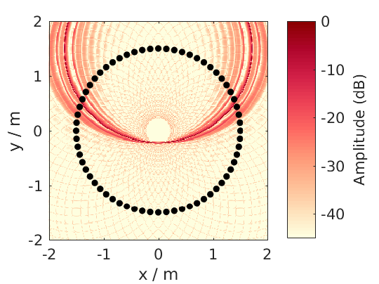
Fig. 19 Sound pressure in decibel of the same broadband impulse point source as in the figure above.
You could change the color map yourself doing the following before the plot command.
conf.plot.colormap = 'jet'; % Matlab rainbow color map
If you want to simulate more than one virtual source, it is a good idea
to set the starting time of your simulation to start with the activity
of your virtual source and not with the secondary sources, which is the
default behavior. You can change this by setting
conf.t0 = 'source'.
conf.plot.useplot = false;
conf.t0 = 'source';
t_40cm = 0.4/conf.c; % time to travel 40 cm in s
t0 = 0.0005; % start time of focused source in s
[p_ps,~,~,~,x0_ps] = ...
    sound_field_imp_wfs([-2 2],[-2 2],0,[1.9 0 0],'ps',t0+t_40cm,conf);
[p_pw,~,~,~,x0_pw] = ...
    sound_field_imp_wfs([-2 2],[-2 2],0,[1 -2 0],'pw',t0-t_40cm,conf);
[p_fs,~,~,~,x0_fs] = ...
    sound_field_imp_wfs([-2 2],[-2 2],0,[0 -1 0 0 1 0],'fs',t0,conf);
plot_sound_field(p_ps+p_pw+p_fs,[-2 2],[-2 2],0,[x0_ps; x0_pw; x0_fs],conf)
hold;
scatter(0,0,'kx');   % origin of plane wave
scatter(1.9,0,'ko'); % point source
scatter(0,-1,'ko');  % focused source
hold off;
%print_png('sound_field_imp_multiple_sources_dB.png');
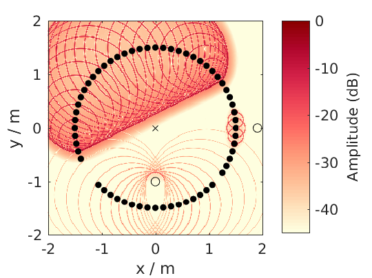
Fig. 20 Sound pressure in decibel of a boradband impulse plane wave, point source, and focused source synthesized all by 2.5D WFS. The plane wave is traveling into the direction (1,-2,0) and shown 0.7 ms before it starting point at (0,0,0). The point source is placed at (1.9,0,0) m and shown 1.7 ms after its start. The focused source is placed at (0,-1,0) m and shown 0.5 ms after its start.