Binaural Simulations

If you have a set of HRTFs or BRIRs you can simulate the ear signals reaching a listener sitting at a given point in the listening area for different spatial audio systems.

In order to easily use different HRTF or BRIR sets the Toolbox uses the SOFA file format. In order to use it you have to install the SOFA API for Matlab/Octave and run SOFAstart before you can use it inside the SFS Toolbox. If you are looking for different HRTFs and BRIRs, a large set of different impulse responses is available: http://www.sofaconventions.org/mediawiki/index.php/Files.

The files dealing with the binaural simulations are in the folder SFS_binaural_synthesis. Files dealing with HRTFs and BRIRs are in the folder SFS_ir. If you want to extrapolate your HRTFs to plane waves you may also want to have a look in the folder SFS_HRTF_extrapolation.

In the following we present some examples of binaural simulations. For their auralization an anechoic recording of a cello is used, which can be downloaded from anechoic_cello.wav.

Binaural simulation of arbitrary loudspeaker arrays

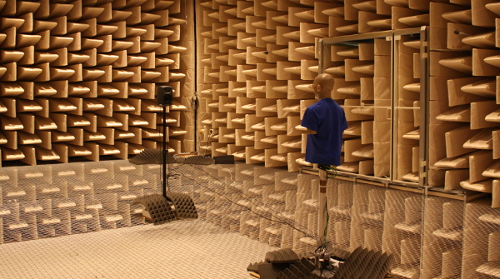
Fig. 22 Setup of the KEMAR and a loudspeaker during a HRTF measurement.

If you use an HRTF data set, it has the advantage that it was recorded in anechoic conditions and the only parameter that matters is the relative position of the loudspeaker to the head during the measurement. This advantage can be used to create every possible loudspeaker array you can imagine, given that the relative locations of all loudspeakers are available in the HRTF data set. The above picture shows an example of a HRTF measurement. You can download the corresponding QU_KEMAR_anechoic_3m.sofa HRTF set, which we can directly use with the Toolbox.

The following example will load the HRTF data set and extracts a single impulse response for an angle of 30° from it. If the desired angle of 30° is not available, a linear interpolation between the next two available angles will be applied. Afterwards the impulse response will be convolved with the cello recording by the auralize_ir() function.

conf = SFS_config;
hrtf = SOFAload('QU_KEMAR_anechoic_3m.sofa');
ir = get_ir(hrtf,[0 0 0],[0 0],[rad(30) 0 3],'spherical',conf);
cello = wavread('anechoic_cello.wav');
sig = auralize_ir(ir,cello,1,conf);
sound(sig,conf.fs);

To simulate the same source as a virtual point source synthesized by WFS and a circular array with a diameter of 3 m, you have to do the following.

conf = SFS_config;
conf.secondary_sources.size = 3;
conf.secondary_sources.number = 56;
conf.secondary_sources.geometry = 'circle';
conf.dimension = '2.5D';
hrtf = SOFAload('QU_KEMAR_anechoic_3m.sofa');
% ir = ir_wfs(X,phi,xs,src,hrtf,conf);
ir = ir_wfs([0 0 0],pi/2,[0 3 0],'ps',hrtf,conf);
cello = wavread('anechoic_cello.wav');
sig = auralize_ir(ir,cello,1,conf);

If you want to use binaural simulations in listening experiments, you should not only have the HRTF data set, but also a corresponding headphone compensation filter, which was recorded with the same dummy head as the HRTFs and the headphones you are going to use in your test. For the HRTFs we used in the last example and the AKG K601 headphones you can download QU_KEMAR_AKGK601_hcomp.wav. If you want to redo the last simulation with headphone compensation, just add the following lines before calling ir_wfs().

conf.ir.usehcomp = true;
conf.ir.hcompfile = 'QU_KEMAR_AKGK601_hcomp.wav';
conf.N = 4096;

The last setting ensures that your impulse response will be long enough for convolution with the compensation filter.

Binaural simulation of a real setup

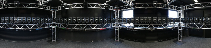
Fig. 23 Boxed shaped loudspeaker array at the University Rostock.

Besides simulating arbitrary loudspeaker configurations in an anechoic space, you can also do binaural simulations of real loudspeaker setups. In the following example we use BRIRs from the 64-channel loudspeaker array of the University Rostock as shown in the panorama photo above. The BRIRs and additional information on the recordings are available for download, see doi:10.14279/depositonce-87.2. For such a measurement the SOFA file format has the advantage to be able to include all loudspeakers and head orientations in just one file.

conf = SFS_config;
brir = 'BRIR_AllAbsorbers_ArrayCentre_Emitters1to64.sofa';
conf.secondary_sources.geometry = 'custom';
conf.secondary_sources.x0 = brir;
conf.N = 44100;
ir = ir_wfs([0 0 0],0,[3 0 0],'ps',brir,conf);
cello = wavread('anechoic_cello.wav');
sig = auralize_ir(ir,cello,1,conf);

In this case, we don’t load the BRIRs into the memory with SOFAload() as the file is too large. Instead, we make use of the ability that SOFA can request single impulse responses from the file by just passing the file name to the ir_wfs() function. In addition, we have to set conf.N to a reasonable large value as this determines the length of the impulse response ir_wfs() will return, which has to be larger as for the anechoic case as it should now include the room reflections. Note, that the head orientation is chosen to be 0 instead of pi/2 as in the HRTF examples due to a difference in the orientation of the coordinate system of the BRIR measurement.

Impulse response of your spatial audio system

Binaural simulations are also an interesting approach to investigate the behavior of a given spatial audio system at different listener positions. Here, we are mainly interested in the influence of the system and not the HRTFs so we simply use a Dirac impulse as HRTF as provided by dummy_irs().

conf = SFS_config;
conf.t0 = 'source';
X = [0 0 0];
phi = 0;
xs = [2.5 0 0];
src = 'ps';
hrtf = dummy_irs(conf);
[ir,~,delay] = ir_wfs(X,phi,xs,src,hrtf,conf);
figure;
figsize(540,404,'px');
plot(ir(1:1000,1),'-g');
hold on;
offset = round(delay*conf.fs);
plot(ir(1+offset:1000+offset,1),'-b');
hold off;
%print_png('img/impulse_response_wfs_25d.png');

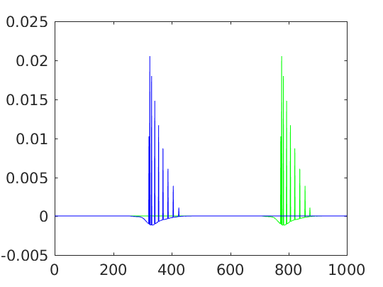
Fig. 24 Sound pressure of an impulse synthesized as a point source by 2.5D WFS at (2.5, 0, 0) m. The sound pressure is observed by a virtual microphone at (0, 0, 0) m. The impulse is plotted including the delay offset of the WFS driving function (green) and with a corrected delay that corresponds to the source poisition (blue).

The figure includes two versions of the impulse response at two different time instances. The green impulse response includes the processing delay that is added by driving_function_imp_wfs() and other functions performing filtering and delaying of signals. This delay is returned by ir_wfs() as well and can be used to correct it during plotting. The blue impulse response is the corrected one, which is now placed at 321 samples which corresponds to the actual distance of the synthesized source of 2.5 m.

The impulse response can also be calculated without involving functions for binaural simulations, but by utilizing directly sound_field_imp() related function.

conf = SFS_config;
    conf.N = 1000;
conf.t0 = 'source';
X = [0 0 0];
phi = 0;
xs = [2.5 0 0];
src = 'ps';
    time_response_wfs(X,xs,src,conf)
%print_png('img/impulse_response_wfs_25d_imp.png');

Fig. 25 Sound pressure of an impulse synthesized as a point source by 2.5D WFS at (2.5, 0, 0) m. The sound pressure is observed by a virtual microphone at (0, 0, 0) m.

This time the delay offset of the driving function is automatically corrected for and the involved calculation uses inherently a fractional delay filter. The downside is that the calculation takes longer and the amplitude is slightly lower by the involved fractional delay method.

Frequency response of your spatial audio system

Binaural simulations are also a nice way to investigate the frequency response of your reproduction system. The following code will investigate the influence of the pre-equalization filter in WFS on the frequency response. For the red line the pre-filter is used and its upper frequency is set to the expected aliasing frequency of the system (above these frequency the spectrum becomes very noise as you can see in the figure).

conf = SFS_config;
conf.ir.usehcomp = false;
conf.wfs.usehpre = false;
hrtf = dummy_irs(conf);
[ir1,x0] = ir_wfs([0 0 0],pi/2,[0 2.5 0],'ps',hrtf,conf);
conf.wfs.usehpre = true;
conf.wfs.hprefhigh = aliasing_frequency(x0,conf);
ir2 = ir_wfs([0 0 0],pi/2,[0 2.5 0],'ps',hrtf,conf);
[a1,p,f] = spectrum_from_signal(norm_signal(ir1(:,1)),conf);
a2 = spectrum_from_signal(norm_signal(ir2(:,1)),conf);
figure;
figsize(540,404,'px');
semilogx(f,20*log10(a1),'-b',f,20*log10(a2),'-r');
axis([10 20000 -80 -40]);
set(gca,'XTick',[10 100 250 1000 5000 20000]);
legend('w/o pre-filter','w pre-filter');
xlabel('frequency / Hz');
ylabel('magnitude / dB');
%print_png('img/frequency_response_wfs_25d.png');

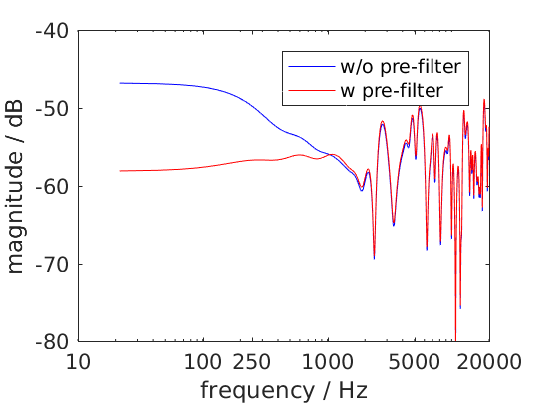
Fig. 26 Sound pressure in decibel of a point source synthesized by 2.5D WFS for different frequencies. The 2.5D WFS is performed with and without the pre-equalization filter. The calculation is performed in the time domain.

The same can be done in the frequency domain, but in this case we are not able to set a maximum frequency of the pre-equalization filter and the whole frequency range will be affected.

freq_response_wfs([0 0 0],[0 2.5 0],'ps',conf);
axis([10 20000 -40 0]);
%print_png('img/frequency_response_wfs_25d_mono.png');

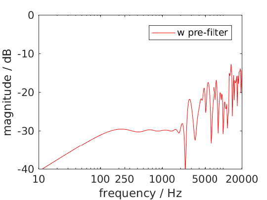
Fig. 27 Sound pressure in decibel of a point source synthesized by 2.5D WFS for different frequencies. The 2.5D WFS is performed only with the pre-equalization filter active at all frequencies. The calculation is performed in the frequency domain.

Using the SoundScape Renderer with the SFS Toolbox

In addition to binaural synthesis, you may want to apply dynamic binaural synthesis, which means you track the position of the head of the listener and switches the used impulse responses regarding the head position. The SoundScape Renderer (SSR) is able to do this. The SFS Toolbox provides functions to generate the needed wav files containing the impulse responses used by the SoundScape Renderer. All functions regarding the SSR are stored in folder SFS_ssr.

conf = SFS_config;
brs = ssr_brs_wfs(X,phi,xs,src,hrtf,conf);
wavwrite(brs,fs,16,'brs_set_for_SSR.wav');